5. Building CC3DML-Based Simulations Using CompuCell3D

To show how to build simulations in CompuCell3D, the reminder of this chapter provides a series of examples of gradually increasing complexity. For each example we provide a brief explanation of the physical and/or biological background of the simulation and listings of the CC3DML configuration file and Python scripts, followed by a detailed explanation of their syntax and algorithms. We begin with three examples using only CC3DML to define simulations.

We use Twedit++-CC3D code generation and explain how to turn automatically-generated draft code into executable models. All of the parameters appearing in the autogenerated simulation scripts are set to their default values.

5.1. Short Introduction to XML

XML is a text-based data-description language, which allows standardized representations of data. XML syntax consists of lists of elements, each either contained between opening (<Tag>) and closing (</Tag>) tags: <Tag Attribute1="text1">ElementText</Tag> or of form <Tag Attribute1="attribute_text1" Attribute2="attribute_text2"/>

We will denote the <Tag>…</Tag> syntax as a <Tag> tag pair. The opening tag of an XML element may contain additional attributes characterizing the element. The content of the XML element (ElementText in the above example) and the values of its attributes (text1, attribute_text1, attribute_text2) are strings of characters. Computer programs that read XML may interpret these strings as other data types such as integers, Booleans or floating point numbers. XML elements may be nested. The simple example below defines an element Cell with subelements (represented as nested XML elements) Nucleus and Membrane assigning the element Nucleus an attribute Size set to “10” and the element Membrane an attribute Area set to “20.5”, and setting the value of the Membrane element to Expanding

 <Cell>
   <Nucleus Size="10"/>
   <Membrane Area="20.5">Expanding</Membrane>
</Cell>

Although XML parsers ignore indentation, all the listings presented in this chapter are block-indented for better readability.

5.2. Cell Sorting Simulation

Cell sorting due to differential adhesion between cells of different types is one of the basic mechanisms creating tissue domains during development and wound healing and in maintaining domains in homeostasis. In a classic in vitro cell sorting experiment to determine relative cell adhesivities in embryonic tissues, mesenchymal cells of different types are dissociated, then randomly mixed and reaggregated. Their motility and differential adhesivities then lead them to rearrange to reestablish coherent homogenous domains with the most cohesive cell type surrounded by the less. The simulation of the sorting of two cell types was the original motivation for the development of GGH methods. Such simple simulations show that the final configuration depends only on the hierarchy of adhesivities, while the sorting dynamics depends on the ratio of the adhesive energies to the amplitude of cell fluctuations.

To invoke the simulation wizard to create a simulation, we click CC3DProject->New CC3D Project in the menu bar. In the initial screen we specify the name of the model (cellsorting), its storage directory (C:\CC3DProjects) and whether we will store the model as pure CC3DML, Python and CC3DML or pure Python. This tutorial will use Python and CC3DML.

Figure 7.: Invoking the CompuCell3D Simulation Wizard from Twedit++

On the next page of the Wizard we specify GGH global parameters, including cell-lattice dimensions, the cell fluctuation amplitude, the duration of the simulation in Monte-Carlo steps and the initial cell-lattice configuration.

In this example, we specify a 100x100x1 cell-lattice, i.e., a 2D model, a fluctuation amplitude of 10, a simulation duration of 10000 MCS and a pixel-copy range of 2. BlobInitializer initializes the simulation with a disk of cells of specified size.

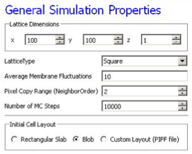
Figure 8.: Specification of basic cell-sorting properties in Simulation Wizard

On the next Wizard page we name the cell types in the model. We will use two cells types: Condensing (more cohesive) and NonCondensing (less cohesive). CC3D by default includes a special generalized-cell type Medium with unconstrained volume which fills otherwise unspecified space in the cell-lattice.

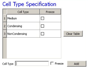
Figure 9.: Specification of cell-sorting cell types in Simulation Wizard.

We skip the Chemical Field page of the Wizard and move to the Cell Behaviors and Properties page. Here we select the biological behaviors we will include in our model. Objects in CC3D have no properties or behaviors unless we specify then explicitly. Since cell sorting depends on differential adhesion between cells, we select the Contact Adhesion module from the Adhesion section and give the cells a defined volume using the Volume Constraint module.

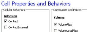
Figure 10.: Selection of cell-sorting cell behaviors in Simulation Wizard.

We skip the next page related to Python scripting, after which Twedit++-CC3D generates the draft simulation code. Double clicking on cellsorting.cc3d opens both the CC3DML (cellsorting.xml) and Python scripts for the model. Because the CC3DML file contains the complete model in this example, we postpone discussion of the Python script. A CC3DML file has 3 distinct sections. The first, the Lattice Section (lines 2-7) specifies global parameters like the cell-lattice size. The Plugin Section (lines 8-30) lists all the plugins used, e.g. CellType and Contact. The Steppable Section (lines 32-39) lists all steppables, here we use only BlobInitializer. Following Simulation-Wizard-generated draft CC3DML (XML) code for cell-sorting-

 <CompuCell3D version="3.6.0">
 <Potts>
  <Dimensions x="100" y="100" z="1"/>
  <Steps>10000</Steps>
  <Temperature>10.0</Temperature>
  <NeighborOrder>2</NeighborOrder>
 </Potts>

 <Plugin Name="CellType">
  <CellType TypeId="0" TypeName="Medium"/>
  <CellType TypeId="1" TypeName="Condensing"/>
  <CellType TypeId="2" TypeName="NonCondensing"/>
 </Plugin>

 <Plugin Name="Volume">
  <VolumeEnergyParameters CellType="Condensing"
     LambdaVolume="2.0" TargetVolume="25"/>
  <VolumeEnergyParameters CellType="NonCondensing"
     LambdaVolume="2.0" TargetVolume="25"/>
 </Plugin>

 <Plugin Name="CenterOfMass"/>

 <Plugin Name="Contact">
  <Energy Type1="Medium" Type2="Medium">10</Energy>
  <Energy Type1="Medium" Type2="Condensing">10</Energy>
  <Energy Type1="Medium" Type2="NonCondensing">10</Energy>
  <Energy Type1="Condensing"Type2="Condensing">10</Energy>
  <Energy Type1="Condensing" Type2="NonCondensing">10</Energy>
  <Energy Type1="NonCondensing" Type2="NonCondensing">10</Energy>
  <NeighborOrder>2</NeighborOrder>
 </Plugin>

 <Steppable Type="BlobInitializer">
  <Region>
   <Center x="50" y="50" z="0"/>
   <Radius>20</Radius>
   <Width>5</Width>
   <Types>Condensing,NonCondensing</Types>
  </Region>
 </Steppable>
</CompuCell3D>

Listing 1: Simulation-Wizard-generated draft CC3DML (XML) code for cell-sorting

Each CC3DML configuration file begins with the <CompuCell3D> tag and ends with the </CompuCell3D> tag. A CC3DML configuration file contains three sections in the following sequence: the lattice section (contained within the`` <Potts>`` tag pair), the plugins section, and the steppables section. The lattice section defines global parameters for the simulation: cell-lattice and field-lattice dimensions (specified using the syntax <Dimensions x="x_dim" y="y_dim" z="z_dim"/>), the number of Monte Carlo Steps to run (defined within the <Steps> tag pair) the effective cell motility (defined within the <Temperature> tag pair) and boundary conditions. The default boundary conditions are no-flux. They can be changed to be periodic along the x and y axes by assigning the value Periodic to the <Boundary_x> and <Boundary_y> tag pairs. The value set by the <NeighborOrder> tag pair defines the range over which source pixels are selected for index-copy attempts (see Figure 4 and Table 1).

The plugins section lists the plugins the simulation will use. The syntax for all plugins which require parameter specification is:

<Plugin Name="PluginName">
  <ParameterSpecification/>
</Plugin>

The CellType plugin is quite special as it does not participate directly in index copies, but is used by other plugins for cell-type-to-cell-index mapping.It uses the parameter syntax

<CellType TypeName="Name" TypeId="IntegerNumber"/>

to map verbose generalized-cell-type names to numeric cell TypeIds for all generalized-cell types. Medium (appearing in Listing 1)is a special cell type with unconstrained volume and surface area that fills all cell-lattice pixels unoccupied by cells of other types.

Steppables section consists of module declaration which follow the following patern:

<Steppable Type="SteppableName" Frequency="FrequencyMCS">
  <ParameterSpecification/>
</Steppable>

The Frequency attribute is optional and by default is 1 MCS.

By autogenerating CC3DML code, Twedit++-CC3D releases user from remembering all the rules necessary to construct a valid CC3DML simulation script. All parameters appearing in the autogenerated CC3DML script have default values inserted by Simulation Wizard. We must edit the parameters in the draft CC3DML script to build a functional cell-sorting model (Listing 1). The CellType plugin (lines 9-13) already provides three generalized-cell types: Condensing (C), NonCondensing (N) and Medium (M), so we need not change it. However, the boundary-energy (Contact-energy) matrix in the Contact plugin (lines 22-30) is initially filled with identical values, i.e., the cell types are identical. For cell-sorting, Condensing cells must adhere strongly to each other (so we set J_CC= 2), Condensing and NonCondensing cells must adhere more weakly (here we set J_CN= 11) and all other adhesion must be very weak (we set J_NN= J_CM= J _NM= 16), as discussed in section. The value of J_MM =0 is irrelevant, since the Medium generalized cell does not contact itself. To reduce artifacts due to the anisotropy of the square cell-lattice we increase the neighbor-order range in the contact energy to 2 so the contact-energy sum in equation () will include nearest and second-nearest neighbors (line 29).

In the Volume plugin, which calculates the Volume-constraint energy given in equation the attributes CellType, LambdaVolume and TargetVolume inside the <VolumeEnergyParameters> tags specify \(\lambda(\tau)\) and \(V_t(\tau)\) for each cell type. In our simulations we set \(V_t(\tau) = 25\) and \(\lambda(\tau) = 2.0\) for both cell types. We initialize the cell lattice using the BlobInitializer, which creates one or more disks (solid spheres in 3D) of cells. Each region is enclosed between`` <Region>`` tags. The`` <Center>`` tag with syntax <Center x="x_position" y="y_position" z= "z_position"/> specifies the position of the center of the disk. The`` <Width>`` tag specifies the size of the initial square (cubical in 3D) generalized cells and the <Gap> tag creates space between neighboring cells. The <Types> tag lists the cell types to fill the disk. Here, we change the Radius in the draft BlobInitializer specification to 40. These few changes produce a working cell-sorting simulation. To run the simulation we right click cellsorting.cc3d in the left panel and choose the Open In Player option. We can also run the simulation by opening CompuCellPlayer and selecting cellsorting.cc3d from the File-> Open Simulation File… dialog.

Figure 11 shows snapshots of a simulation of the cell-sorting model. The less cohesive NonCondensing cells engulf the more cohesive Condensing cells, which cluster and form a single central domain. By changing the boundary energies we can produce other cell-sorting patterns. In particular, if we reduce the contact energy between the Condensing cell type and the Medium, we can force inverted cell sorting, where the Condensing cells surround the NonCondensing cells. If we set the heterotypic contact energy to be less than either of the homotypic contact energies, the cells of the two types will mix rather than sort. If we set the cell-medium contact energy to be very small for one cell type, the cells of that type will disperse into the medium, as in cancer invasion. With minor modifications, we can also simulate the scenarios for three or more cell types, for situations in which the cells of a given type vary in volume, motility or adhesivity, or in which the initial condition contains coherent clusters of cells rather than randomly mixed cells (engulfment).

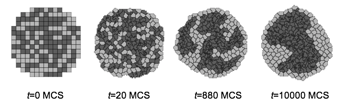
Figure 11.: Snapshots of the cell-lattice configurations for the cell-sorting simulation in Listing 1. The boundary-energy hierarchy drives NonCondensing (light grey) cells to surround Condensing (dark grey) cells. The white background denotes surrounding Medium

5.3. Angiogenesis Model

Vascular development is central to both development and cancer progression. We present a simplified model of the earliest phases of capillary network assembly by endothelial cells based on cell adhesion and contact-inhibited chemotaxis. This model does a good job of reproducing the patterning and dynamics which occur if we culture Human Umbilical Vein Endothelial Cells (HUVEC) on matrigel in a quasi-2D in vitro experiment (Merks and Glazier 2006, Merks et al., 2006, 2008). In addition to generalized cells modeling the HUVEC, we will need a diffusing chemical object, here, Vascular Endothelial Growth Factor (VEGF), cell secretion of VEGF and cell-contact-inhibited chemotaxis to VEGF.

We will use a 3D voxel (pixel) with a side of 4 µm, i.e. a volume of 64 µm³. Since the experimental HUVEC speed is about 0.4 µm/min and cells in this simulation move at an average speed of 0.1 pixel/MCS, one MCS represents one minute.

In the Simulation Wizard, we name the model ANGIOGENESIS, set the cell- and field-lattice dimensions to 50×50×50, the membrane fluctuation amplitude to 20, the pixel-copy range to 3, the number of MCS to 10000 and select BlobFieldInitializer to produce the initial cell-lattice configuration. We have only one cell type – Endothelial.

In the Chemical Fields page we create the VEGF field and select FlexibleDiffusionSolverFE from the Solver pull-down list.

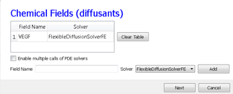
Figure 12.: Specification of the angiogenesis chemical field in Simulation Wizard

Next, on the Cell Properties and Behaviors page, we select the Contact module from the Adhesion-behavior group and add Secretion, Chemotaxis and Volume-constraint behaviors by checking the appropriate boxes.

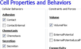
Figure 13.: Specification of angiogenesis cell behaviors in Simulation Wizard

Because we have invoked Secretion and Chemotaxis, the Simulation Wizard opens their configuration screens. On the Secretion page, from the pull-down list, we select the chemical to secrete by selecting VEGF in the Field pull-down menu and the cell type secreting the chemical (Endothelial), and enter the rate of 0.013 (50 pg (cell h)^-1= 0.013 pg (voxel MCS)^-1, compare to Leith and Michelson 1995). We leave the Secretion Type entry set to Uniform, so each pixel of an endothelial cell secretes the same amount of VEGF at the same rate. Uniform volumetric secretion or secretion at the cell’s center of mass may be most appropriate in 2D simulations of planar geometries (e.g. cells on a petrie dish or agar) where the biological cells are actually secreting up or down into a medium that carries the diffusant. CC3D also supplies a secrete-on-contact option to secrete outwards from the cell boundaries and allows specification of which boundaries can secrete, which is more realistic in 3D. However, users are free to employ any of these methods in either 2D or 3D depending on their interpretation of their specific biological situation. CompuCell3D does not have intrinsic units for fields, so the amount of a chemical can be interpreted in units of moles, number of molecules or grams. We click the Add Entry button to add the secretion information, then proceed to the next page to define the cells’ chemotaxis properties.

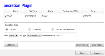
Figure 14.: Specification of angiogenesis secretion parameters in Simulation Wizard

On the Chemotaxis page, we select VEGF from the Field pull-down list and Endothelial for the cell type, entering a value for Lambda of 5000. When the chemotaxis type is regular, the cell’s response to the field is linear, i.e. the effective strength of chemotaxis depends on the product of Lambda and the secretion rate of VEGF, e.g. a Lambda of 5000 and a secretion rate of 0.013 has the same effective chemotactic strength as a Lambda of 500 and a secretion rate of 0.13. Since endothelial cells do not chemotax at surfaces where they contact other endothelial cells (contact-inhibition), we select Medium from the pull-down menu next to the Chemotax Towards button and click this button to add Medium to the list of generalized cell types whose interfaces with Endothelial cells support chemotaxis. We click the Add Entry button to add the chemotaxis information, then proceed to the final Simulation Wizard page.

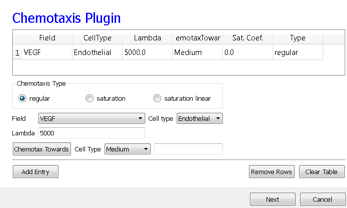
Figure 15.: Specification of angiogenesis chemotaxis properties in Simulation Wizard

Next, we adjust the parameters of the draft model. Pressure from chemotaxis to VEGF reduces the average endothelial-cell volume by about 10 voxels from the target volume. So, in the Volume plugin we set TargetVolume to 74 (64+10) and LambdaVolume to 20.0. In experiments, in the absence of chemotaxis no capillary network forms and cells adhere to each other to form clusters. We therefore set J_MM=0, J_EM=12 and J_EE=5 in the Contact plugin (M: Medium, E: Endothelial). We also set the NeighborOrder for the Contact energy calculations to 4.

The diffusion equation that governs VEGF ( \(V(x)\)) field evolution is:

\[{\delta V(\vec{x}) \over{\delta t}} = D^{EC}_{VEGF} \bigtriangledown^2 V(\vec{x}) - \gamma_{VEGF} V(\vec{x}) \delta(\tau(\sigma(\vec{x}), M) + S^{EC} \delta(\tau(\sigma(\vec{x})), EC)\]

where, \(\delta(\tau(\sigma(\vec{x})), EC)=1\) inside Endothelial cells and 0 elsewhere and \(\delta(\tau(\sigma(\vec{x}), M)=1\) inside medium and 0 elsewhere. We set the diffusion constant \(D_{VEGF}=0.042 µm^2/sec\) (0.16 voxel ²/MCS, about two orders of magnitude smaller than experimental values) [1], the decay coefficient \(\gamma_{VEGF} =1 h^{-1}\) [130,131] (0.016 MCS-1) for Medium pixels and \(\gamma_{VEGF}=0\) inside Endothelial cells, and the secretion rate \(S^{EC}=0.013\) pg (voxel MCS):sup:-1. In the CC3DML script describing FlexibleDiffusionSolverFE (Listing 2, lines 38-47) we set the values of the <DiffusionConstant> and <DecayConstant> tags to 0.16 and 0.016 respectively. To prevent chemical decay inside Endothelial cells we add the line <DoNotDecayIn>Endothelial</DoNotDecayIn> inside the <DiffusionData> tag pair. Finally, we edit BlobInitializer (lines 49-56) to start with a solid sphere 10 pixels in radius centered at x=25, y=25, z=25 with initial cell width 4, as following-

  <CompuCell3D version="3.6.0">

  <Potts>
   <Dimensions x="50" y="50" z="50"/>
   <Steps>10000</Steps>
   <Temperature>20.0</Temperature>
   <NeighborOrder>3</NeighborOrder>
  </Potts>

  <Plugin Name="CellType">
   <CellType TypeId="0" TypeName="Medium"/>
   <CellType TypeId="1" TypeName="Endothelial"/>
  </Plugin>

  <Plugin Name="Volume">
   <VolumeEnergyParameters CellType="Endothelial"
      LambdaVolume="20.0" TargetVolume="74"/>
  </Plugin>

  <Plugin Name="Contact">
   <Energy Type1="Medium" Type2="Medium">0</Energy>
   <Energy Type1="Medium" Type2="Endothelial">12</Energy>
   <Energy Type1="Endothelial" Type2="Endothelial">5</Energy>
   <NeighborOrder>4</NeighborOrder>
  </Plugin>

  <Plugin Name="Chemotaxis">
   <ChemicalField Name="VEGF" Source="FlexibleDiffusionSolverFE">
    <ChemotaxisByType ChemotactTowards="Medium" Lambda="5000.0"
       Type="Endothelial"/>
   </ChemicalField>
  </Plugin>

  <Plugin Name="Secretion">
   <Field Name="VEGF">
    <Secretion Type="Endothelial">0.013</Secretion>
   </Field>
  </Plugin>

  <Steppable Type="FlexibleDiffusionSolverFE">
   <DiffusionField>
    <DiffusionData>
     <FieldName>VEGF</FieldName>
     <DiffusionConstant>0.16</DiffusionConstant>
     <DecayConstant>0.016</DecayConstant>
     <DoNotDecayIn> Endothelial</DoNotDecayIn>
    </DiffusionData>
   </DiffusionField>
  </Steppable>

  <Steppable Type="BlobInitializer">
  <Region>
  <Center x="25" y="25" z="25"/>
    <Radius>10</Radius>
    <Width>4</Width>
    <Types>Endothelial</Types>
  </Region>
  </Steppable>

  </CompuCell3D>

Listing 2: CC3DML code for the angiogenesis model.

The main behavior that drives vascular patterning is contact-inhibited chemotaxis (Listing 2, lines 26-30). VEGF diffuses away from cells and decays in Medium, creating a steep concentration gradient at the interface between Endothelial cells and Medium. Because Endothelial cells chemotax up the concentration gradient only at the interface with Medium the Endothelial cells at the surface of the cluster compress the cluster of cells into vascular branches and maintain branch integrity. We show screenshots of a simulation of the angiogenesis model in Figure 16 [Merks et al., 2008, Shirinifard et al., 2009]. We can reproduce either 2D or 3D primary capillary network formation and the rearrangements of the network agree with experimentally-observed dynamics. If we eliminate the contact inhibition, the cells do not form a branched structure (as observed in chick allantois experiments, Merks et al., 2008). We can also study the effects of surface tension, external growth factors and changes in motility and diffusion constants on the pattern and its dynamics. However, this simple model does not include the strong junctions HUVEC cells make with each other at their ends after a period of prolonged contact. It also does not attempt to model the vacuolation and linking of vacuoles that leads to a connected network of tubes.

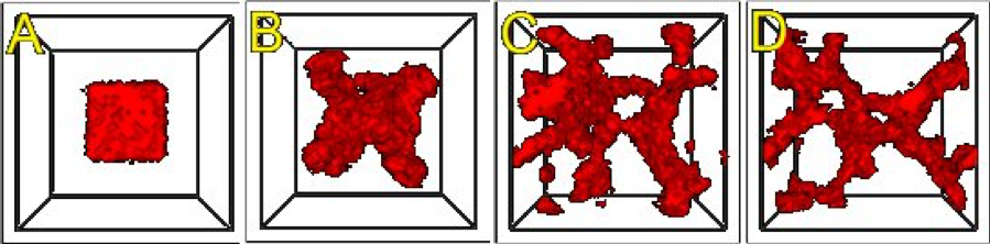
Figure 16.: An initial cluster of adhering endothelial cells forms a capillary-like network via sprouting angiogenesis. A: 0 hours (0 MCS), B: ~2 hours (100 MCS), C: ~5 hours (250 MCS), D: ~18 hours (1100 MCS).

Since real endothelial cells are elongated, we can include the Cell-elongation plugin in the Simulation Wizard to better reproduce individual cell morphology. However, excessive cell elongation causes cell fragmentation. Adding either the Global or Fast Connectivity Constraint plugin prevents cell fragmentation.

[1]	FlexibleDiffusionSolverFE becomes unstable for values of :math:’D_{VEGF}>0.16 voxel2/MCS’. For larger diffusion constants we must call the algorithm multiple times per MCS (See the Three-Dimensional Vascular Solid Tumor Growth section).

5.4. Bacterium-and-Macrophage Simulation

Another example which illustrates the use of chemical fields is based on the in vitro behavior of bacteria and macrophages in blood. In the famous experimental movie taken in the 1950s by David Rogers at Vanderbilt University, the macrophage appears to chase the bacterium, which seems to run away from the macrophage. We can model both behaviors using cell secretion of diffusible chemical signals and movement of the cells in response to the chemical (chemotaxis): the bacterium secretes a signal (a chemoattractant) that attracts the macrophage and the macrophage secretes a signal (a chemorepellant) which repels the bacterium (97). The basic procedure to construct the simulation is very similar to the one we followed in constructing angiogenesis model.

In Twedit++-CC3D we open new project and name it bacterium_macrophage. We declare 3 cell types – Bacterium, Macrophage and Red (red blood cells). We assume that diffusing chemoattractant is secreted by bacteria, therefore on the Chemical Field page of the Simulation Wizard we declare ATTR chemical field which we will solve using DiffusionSolverFE. On the Cell Behaviors and Properties page we select Contact, Chemotaxis, VolumeFlex and Surface Flex. Clicking ‘Next’ button brings us to chemotaxis page where we set chemotaxis parameters as shown on Figure 17:

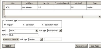
Figure 17.: Setting up chemotaxis properties forMacrophages

After code-autogenerating is done we have to do several adjustments to the CC3DML script.

<CompuCell3D version="3.6.2">

   <Potts>
      <Dimensions x="100" y="100" z="1"/>
      <Steps>10000</Steps>
      <Temperature>40.0</Temperature>
      <NeighborOrder>2</NeighborOrder>
      <Boundary_x>Periodic</Boundary_x>
      <Boundary_y>Periodic</Boundary_y>
   </Potts>

   <Plugin Name="CellType">
      <CellType TypeId="0" TypeName="Medium"/>
      <CellType TypeId="1" TypeName="Bacterium"/>
      <CellType TypeId="2" TypeName="Macrophage"/>
      <CellType TypeId="3" TypeName="Red"/>
   </Plugin>

   <Plugin Name="Volume">
<VolumeEnergyParameters CellType="Bacterium" LambdaVolume="60.0" TargetVolume="10"/>
      <VolumeEnergyParameters CellType="Macrophage" LambdaVolume="15.0" TargetVolume="150"/>
      <VolumeEnergyParameters CellType="Red" LambdaVolume="30.0" TargetVolume="100"/>
   </Plugin>

   <Plugin Name="Surface">
      <SurfaceEnergyParameters CellType="Bacterium" LambdaSurface="4.0" TargetSurface="10"/>
      <SurfaceEnergyParameters CellType="Macrophage" LambdaSurface="20.0" TargetSurface="50"/>
      <SurfaceEnergyParameters CellType="Red" LambdaSurface="0.0" TargetSurface="40"/>
   </Plugin>

   <Plugin Name="Contact">
      <Energy Type1="Medium" Type2="Medium">10.0</Energy>
      <Energy Type1="Medium" Type2="Bacterium">8.0</Energy>
      <Energy Type1="Medium" Type2="Macrophage">8.0</Energy>
      <Energy Type1="Medium" Type2="Red">30.0</Energy>
      <Energy Type1="Bacterium" Type2="Bacterium">150.0</Energy>
      <Energy Type1="Bacterium" Type2="Macrophage">15.0</Energy>
      <Energy Type1="Bacterium" Type2="Red">150.0</Energy>
      <Energy Type1="Macrophage" Type2="Macrophage">150.0</Energy>
      <Energy Type1="Macrophage" Type2="Red">150.0</Energy>
      <Energy Type1="Red" Type2="Red">150.0</Energy>
      <NeighborOrder>2</NeighborOrder>
   </Plugin>

   <Plugin Name="Chemotaxis">
      <ChemicalField Name="ATTR" Source="DiffusionSolverFE">
         <ChemotaxisByType Lambda="1.0" Type="Macrophage"/>
      </ChemicalField>
   </Plugin>

   <Steppable Type="DiffusionSolverFE">
      <DiffusionField>
         <DiffusionData>
            <FieldName>ATTR</FieldName>
            <GlobalDiffusionConstant>0.1</GlobalDiffusionConstant>
            <GlobalDecayConstant>5e-05</GlobalDecayConstant>
            <DiffusionCoefficient CellType="Red">0.0</DiffusionCoefficient>
         </DiffusionData>
         <SecretionData>
            <Secretion Type="Bacterium">100</Secretion>
         </SecretionData>
         <BoundaryConditions>
            <Plane Axis="X">
               <Periodic/>
            </Plane>
            <Plane Axis="Y">
               <Periodic/>
            </Plane>
         </BoundaryConditions>
      </DiffusionField>
   </Steppable>

   <Steppable Type="PIFInitializer">
      <PIFName>Simulation/bacterium_macrophage.piff</PIFName>
   </Steppable>

</CompuCell3D>

Listing 3: CC3DML code for Bacterium Macrophage simulation. Note that the code has been modified from its autogenetrated version

We implement the actual bacterium-macrophage “chasing” mechanism using the Chemotaxis plugin, which specifies how a generalized cell of a given type responds to a field. The Chemotaxis plugin biases a cell’s motion up or down a field gradient by changing the calculated effective-energy change used in the acceptance function, equation (7). For a field \(c(i)\) :

\[\Delta H_{chem} = - \lambda_{chem} (c(i) - c(i'))\]

where \(c(i)\) is the chemical field at the index-copy target pixel, \(c(i')\) the field at the index-copy source pixel, and \(\lambda_{chem}\) the strength and direction of chemotaxis. If \(\lambda_{chem}\) and \(c(i) > c(i')\) , then \(\Delta H_{chem}\) is negative, increasing the probability of accepting the index copy in equation (7). The net effect is that the cell moves up the field gradient with a velocity \(~\lambda_{chem} \bigtriangledown c\). If \(\lambda < 0\) is negative, the opposite occurs, and the cell will move down the field gradient. Plugins with more sophisticated \(\Delta H_{chem}\) calculations (e.g., including response saturation) are available within CompuCell3D (see the description of the chemotaxis plugin in the second part of this manual).

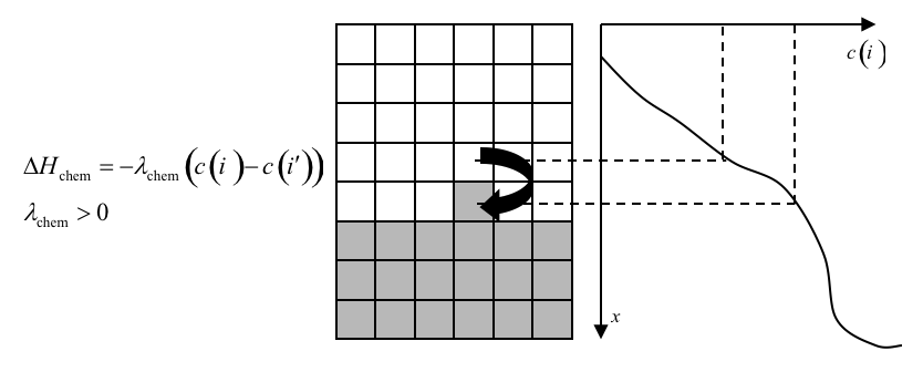
Figure 18: Connecting a field to GGH dynamics using a chemotaxis-energy term. The difference in the value of the field at the source, , and target, , pixels changes the of the index-copy attempt. Here and , so , increasing the probability of accepting the index-copy attempt in equation (7).

In the Chemotaxis plugin we must identify the names of the fields, where the field information is stored, the list of the generalized-cell types that will respond to the fields, and the strength and direction of the response (\(Lambda = \lambda_{chem}\)). The information for each field is specified using the syntax:

<ChemicalField Source="where field is stored" Name="field name">
   <ChemotaxisByType Type="cell_type1" Lambda="lambda1"/>
   <ChemotaxisByType Type="cell_type2" Lambda="lambda1"/>
</ChemicalField>

In our current example, the first field, named ATTR, is stored in DiffusionSolverFE. Macrophage cells are attracted to ATTR with \(\lambda_{chem}=1\). None of the other cell types responds to ATTR. Similarly, Bacterium cells are repelled by REP with \(\lambda_{chem}=-0.1\).

Keep in mind that fields are not created within the Chemotaxis plugin, which only specifies how different cell types respond to the fields. We define and store the fields elsewhere. Here, we use the DiffusionSolverFE steppable as the source of our fields. The DiffusionSolverFE steppable is the main CompuCell3D tool for defining diffusing fields, which evolve according to the diffusion equation:

\[{\delta c(i)\over{\delta t}} = D(i) \nabla^2c(i) - k(i)c(i)+s(i)\]

where \(c(i)\) is the field concentration \(D(i)\), \(k(i)\) and \(s(i)\) denote the diffusion constant (in m:sup:2/s), decay constant (in s:sup:-1) and secretion rates (in concentration/s) of the field, respectively. \(D(i)\), \(k(i)\) and \(s(i)\) may vary with position and cell-lattice configuration. As in the Chemotaxis plugin, we may define the behaviors of multiple fields, enclosing each one within <DiffusionField> tag pairs. For each field defined within a <DiffusionData> tag pair, users provide values for the name of the field (using the <FieldName> tag pair), the global diffusion constant (using the <GlobalDiffusionConstant> tag pair) , and the global decay constant (using the <GlobalDiffusionConstant> tag pair). We can also specify diffusion constant for particular cell types using the following syntax:

<DiffusionCoefficient CellType="cell_type_1">coefficient</DiffusionCoefficient>
<DecayCoefficient CellType="cell_type_1">coefficient</DecayCoefficient>

Forward-Euler methods are numerically unstable for large diffusion constants, limiting the maximum nominal diffusion constant allowed in CompuCell3D simulations. However, by increasing the PDE-solver calling frequency, which reduces the effective time step, CompuCell3D can simulate arbitrarily large diffusion constants and using the DiffusionSolverFE to solve diffusion equation releases users from specifying how many extra times the solver needs to be called.

The optional <SecretionData> tag pair defines a subsection which identifies cells types that secrete or absorb the field and the rates of secretion:

<SecretionData>
   <Secretion Type="cell_type1">real_rate1</Secretion>
   <Secretion Type="cell_type2">real_rate2</Secretion>
<SecretionData>

A negative rate simulates absorption. In the bacterium and macrophage simulation, Bacterium cells secrete ATTR.

To complete specification of the PDE diffusion equation we also set boundary conditions (by default they are set to no flux). Here however we set them to Periodic along x and y directions using the following syntax:

<BoundaryConditions>
   <Plane Axis="X">
     <Periodic/>
     </Plane>
   <Plane Axis="Y">
     <Periodic/>
   </Plane>
</BoundaryConditions>

We load the initial configuration for the bacterium-and-macrophage simulation using the PIFInitializer steppable. Many simulations require initial generalized-cell configurations that we cannot easily construct from primitive regions filled with cells using BlobInitializer and UniformInitializer. To allow maximum flexibility, CompuCell3D can read the initial cell-lattice configuration from Pixel Initialization Files (PIFFs). A PIFF is a text file that allows users to assign multiple rectangular (parallelepiped in 3D) pixel regions or single pixels to particular cells. Each line in a PIF has the syntax:

Cell_id Cell_type x_low x_high y_low y_high z_low z_high

where Cell_id is a unique cell index. A PIF may have multiple, possibly non-adjacent, lines starting with the same Cell_id; all lines with the same Cell_id define pixels of the same generalized cell. The values x_low, x_high, y_low, y_high, z_low and z_high define rectangles (parallelepipeds in 3D) of pixels belonging to the cell. In the case of overlapping pixels, a later line overwrites pixels defined by earlier lines. The following line describes a 6 x 6-pixel square cell with cell index 0 and type Amoeba:

0 Amoeba 10 15 10 15 0 0

If we save this line to the file ‘amoebae.piff’, we can load it into a simulation using the following syntax:

<Steppable Type="PIFInitializer">
 <PIFName>amoebae.piff</PIFName>
</Steppable>

Listing 4 illustrates how to construct arbitrary shapes using a PIF. Here we define two cells with indices 0 and 1, and cell types Amoeba and Bacterium, respectively. The main body of each cell is a 6 x 6 square to which we attach additional pixels.

0 Amoeba 10 15 10 15 0 0
1 Bacterium 25 30 25 30 0 0
0 Amoeba 16 16 15 15 0 0
1 Bacterium 25 27 31 35 0 0

Listing 4. Simple PIF initializing two cells, one each of type Bacterium and Amoeba.

All lines with the same cell index (first column) define a single cell. Figure 19 shows the initial cell-lattice configuration specified in Listing 4:

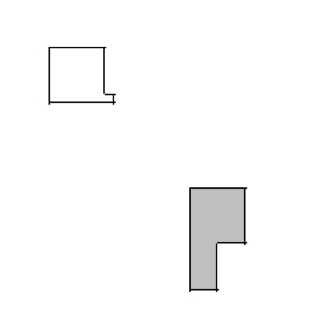
Figure 19: Initial configuration of the cell lattice based on the PIF in Listing 4.

In practice, because constructing complex PIFs by hand is cumbersome, we generally use custom-written scripts to generate the file directly, or convert images stored in graphical formats (e.g., gif, jpeg, png) from experiments or other programs.

Listing 5 shows the example PIF for the bacterium-and-macrophage simulation.

0 Red 10 20 10 20 0 0
1 Red 10 20 40 50 0 0
2 Red 10 20 70 80 0 0
3 Red 40 50 0 10 0 0
4 Red 40 50 30 40 0 0
5 Red 40 50 60 70 0 0
6 Red 40 50 90 95 0 0
7 Red 70 80 10 20 0 0
8 Red 70 80 40 50 0 0
9 Red 70 80 70 80 0 0
11 Bacterium 5 5 5 5 0 0
12 Macrophage 35 35 35 35 0 0
13 Bacterium 65 65 65 65 0 0
14 Bacterium 65 65 5 5 0 0
15 Bacterium 5 5 65 65 0 0
16 Macrophage 75 75 95 95 0 0
17 Red 24 28 10 20 0 0
18 Red 24 28 40 50 0 0
19 Red 24 28 70 80 0 0
20 Red 40 50 14 20 0 0
21 Red 40 50 44 50 0 0
22 Red 40 50 74 80 0 0
23 Red 54 59 90 95 0 0
24 Red 70 80 24 28 0 0
25 Red 70 80 54 59 0 0
26 Red 70 80 84 90 0 0
27 Macrophage 10 10 95 95 0 0

Listing 5. PIF defining the initial cell-lattice configuration for the bacterium-and-macrophage simulation. The file is stored as ‘bacterium_macrophage_2D_wall_v3.pif’.

In Error! Reference source not found. we read the cell lattice configuration from the file ‘bacterium_macrophage_2D_wall_v3.pif’ using the lines:

<Steppable Type="PIFInitializer">
 <PIFName>Simulation/bacterium_macrophage.piff</PIFName>
</Steppable>

Figure 20 shows snapshots of the bacterium-and-macrophage simulation. By adjusting the properties and number of bacteria, macrophages and red blood cells and the diffusion properties of the chemical fields, we can build a surprisingly good reproduction of the experiment.

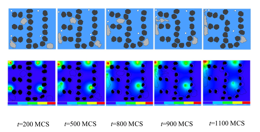
Figure 20. Snapshots of the bacterium-and-macrophage simulation from Error! Reference source not found. and the PIF in Listing 5 saved in the file ‘bacterium_macrophage_2D_wall_v3.pif’. The upper row shows the cell-lattice configuration with the Macrophages in grey, Bacteria in white, red blood cells in dark grey and Medium in blue. Second row shows the concentration of the chemoattractant ATTR secreted by the Bacteria. The bars at the bottom of the field images show the concentration scales (blue, low concentration, red, high concentration).